28. Classical and Quantum Probability Theory
While a classical bit which is binary can thought of as a an unbiased coinflip Heads \((H)\) or Tails \((T)\) with
A quantum bit on the other hand, or more famously a qubit, could be visualised as a spinning coin that hasn’t decided yet. While it’s spinning, from the naked eyes it looks like a sphere
29. Quantum Machine Learning is a rocket emerging
While Machine learning is how classical computers learn patterns in data. Quantum machine learning on the other hand is about how Quantum Computers and other quantum information processors can learn patterns in data that is impossible for classical machine learning algorithms to learne.
The notions and properties of calssical probability distributions can be distinguished from Quantum states. can be thought of as with certain properties that can be distinguished from our classical notion of probabilities. By contrasting these two properties, we can straightforwardly and easily formulate some of the most basic concepts needed in quantum computing.
Alongside probability theory, linear algebra is also crucially important for many learning protocols. In quantum computing is in general all about linear algebra. We will demonstrate how intrinsically linked quantum computing, geometry and probabilities are. Geometric notions are also familiarity in dealing with classical probability distributions. This notebook first talks about classical probabilities and stochastic vectors, and introduces quantum states as a natural generalization.
Throughout this course, we will assume finite probability distributions and finite dimensional spaces. This significantly simplifies notation and most quantum computers operate over finite dimensional spacese, so we do not lose much in generality.
Throughout the following chapters we will assume finite probability distributions and finite dimensional spaces. This significantly simplifies notation and most quantum computers operate over finite dimensional spaces, so we do not lose much in generality.
We’ve introduced quantum states as a generalization of classical probability distributions and quantum computations as a way of transforming these probability distributions. Before we get to quantum states and quantum computations, let’s look at a couple of elements of classical probability theory. So let’s start by looking at coin flipping. so coin flipping has two possible outcomes– heads or tails. And we associate the probability with each of these outcomes some P0 probability with heads and P1 with tails.
Classical probability distributions can be thought of as a special case of the more generalized quantum states, and quantum computation is the way of transforming these probability distributions. Before diving into quantum states and quantum computations, let’s exploit some classical probability theory elements. A coin flip is an instructive starting point where we have two possible outcomes - heads or tails, associated with equally probable outcomes where p0 is the probability for heads and p1 for tails. More formally the probability for the outcome X to be H which is head is p0, and the same for tails T
Probability theory is a cornerstone for machine learning. We can think of quantum states as probability distributions with certain properties that make them different from our classical notion of probabilities. Contrasting these properties is an easy and straightforward introduction to the most basic concepts we need in quantum computing.
Apart from probability theory, linear algebra is also critical for many learning protocols. As we will see, geometry and probabilities are intrinsically linked in quantum computing, but geometric notions are also familiar in dealing with classical probability distributions. This notebook first talks about classical probabilities and stochastic vectors, and introduces quantum states as a natural generalization.
Throughout this course, we will assume finite probability distributions and finite dimensional spaces. This significantly simplifies notation and most quantum computers operate over finite dimensional spaces, so we do not lose much in generality.
30. Classical probability distributions
Let us toss a biased coin. Without getting too technical, we can associate a random variable \(X\) with the output: it takes the value 0 for heads and the value 1 for tails. We get heads with probability \(P(X=0) = p_0\) and tails with \(P(X=1) = p_1\) for each toss of the coin. In classical, Kolmogorovian probability theory, \(p_i\geq 0\) for all \(i\), and the probabilities sum to one: \(\sum_i p_i = 1\). Let’s sample this distribution
import numpy as np
N = 100
p_1 = 0.2
x_data = np.random.binomial(1, p_1, (N,))
print(x_data)
[1 0 0 0 0 0 0 0 0 0 0 0 1 0 1 1 0 0 0 0 0 0 0 0 0 0 1 0 0 1 0 1 0 1 0 0 0
 0 0 1 1 0 0 0 0 0 0 0 0 0 0 0 0 0 0 1 0 0 0 0 0 0 0 0 0 0 0 0 0 0 0 1 0 1
 0 0 0 0 0 0 0 0 0 1 0 0 1 1 1 1 0 0 0 1 0 0 0 0 0 0]
type(x_data)
numpy.ndarray
x_data.sum()
19
def flip(p, N):
    return 'H' if np.random.random() < p else 'T'
flips = [flip(0.5, 150) for i in np.arange(N)]
float(flips.count('H'))/N
0.45
flips = [flip(0.5, 150) for i in np.arange(N)]
float(flips.count('H'))/N
0.47
len(flips)
100
flips[3]
'T'
def remove(string):
    return string.replace(" ", "")

dict = {'a': '1',
    'b': '2',
    'c': '3',
    'd': '4',
    'e': '5',
    'f': '6',
    'g': '7',
    'h': '8',
    'i': '9',
    'j': '10',
    'k': '11',
    'l': '12',
    'm': '13',
    'n': '14',
    'o': '15',
    'p': '16',
    'q': '17',
    'r': '18',
    's': '19',
    't': '20',
    'u': '21',
    'v': '22',
    'w': '23',
    'x': '24',
    'y': '25',
    'z': '26',
}

word = remove(input(''))

for x in word:
    print(dict[x])
---------------------------------------------------------------------------
StdinNotImplementedError                  Traceback (most recent call last)
Cell In[9], line 32
      2     return string.replace(" ", "")
      4 dict = {'a': '1',
      5     'b': '2',
      6     'c': '3',
   (...)
     29     'z': '26',
     30 }
---> 32 word = remove(input(''))
     34 for x in word:
     35     print(dict[x])

File ~/micromamba/envs/mom1env/lib/python3.8/site-packages/ipykernel/kernelbase.py:1190, in Kernel.raw_input(self, prompt)
   1188 if not self._allow_stdin:
   1189     msg = "raw_input was called, but this frontend does not support input requests."
-> 1190     raise StdinNotImplementedError(msg)
   1191 return self._input_request(
   1192     str(prompt),
   1193     self._parent_ident["shell"],
   1194     self.get_parent("shell"),
   1195     password=False,
   1196 )

StdinNotImplementedError: raw_input was called, but this frontend does not support input requests.
index = 0
for x in word:
   print(dict[word[index]])
   index = index + 1
23
import matplotlib.pyplot as plt
# for inline plots in jupyter
%matplotlib inline
# import matplotlib
import matplotlib.pyplot as plt
# for latex equations
from IPython.display import Math, Latex
# for displaying images
from IPython.core.display import Image
# import seaborn
import seaborn as sns
# settings for seaborn plotting style
sns.set(color_codes=True)
# settings for seaborn plot sizes
sns.set(rc={'figure.figsize':(5,5)})
from scipy.stats import norm
# generate random numbers from N(0,1)
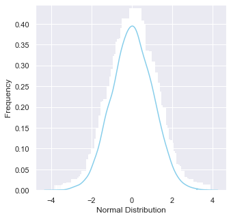
data_normal = norm.rvs(size=10000,loc=0,scale=1)
ax = sns.distplot(data_normal,
                  bins=100,
                  kde=True,
                  color='skyblue',
                  hist_kws={"linewidth": 15,'alpha':1})
ax.set(xlabel='Normal Distribution', ylabel='Frequency')
/Library/Frameworks/Python.framework/Versions/3.10/lib/python3.10/site-packages/seaborn/distributions.py:2619: FutureWarning: `distplot` is a deprecated function and will be removed in a future version. Please adapt your code to use either `displot` (a figure-level function with similar flexibility) or `histplot` (an axes-level function for histograms).
  warnings.warn(msg, FutureWarning)
[Text(0.5, 0, 'Normal Distribution'), Text(0, 0.5, 'Frequency')]
#[Text(0,0.5,u'Frequency'), Text(0.5,0,u'Normal Distribution')]
https://www.kaggle.com/nowke9/statistics-2-distributions
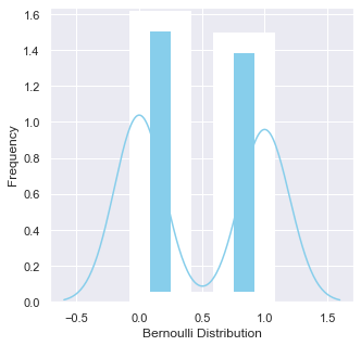
from scipy.stats import bernoulli
data_bern = bernoulli.rvs(size=100,p=0.5)
ax= sns.distplot(data_bern,
                 kde=True, #False
                 color="skyblue",
                 hist_kws={"linewidth": 19,'alpha':1})
ax.set(xlabel='Bernoulli Distribution', ylabel='Frequency')
/Library/Frameworks/Python.framework/Versions/3.10/lib/python3.10/site-packages/seaborn/distributions.py:2619: FutureWarning: `distplot` is a deprecated function and will be removed in a future version. Please adapt your code to use either `displot` (a figure-level function with similar flexibility) or `histplot` (an axes-level function for histograms).
  warnings.warn(msg, FutureWarning)
[Text(0.5, 0, 'Bernoulli Distribution'), Text(0, 0.5, 'Frequency')]
https://www.datacamp.com/community/tutorials/probability-distributions-python
End Test
We naturally expect that the empirically observed frequencies also sum to one:
frequency_of_zeros, frequency_of_ones = 0, 0
for x in x_data:
    if x:
        frequency_of_ones += 1/n_samples
    else:
        frequency_of_zeros += 1/n_samples
print(frequency_of_ones+frequency_of_zeros)
1.0000000000000004
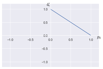
Since \(p_0\) and \(p_1\) must be non-negative, all possible probability distributions are restricted to the positive orthant. The normalization constraint puts every possible distribution on a straight line. This plot describes all possible probability distributions by biased and unbiased coins.
import matplotlib.pyplot as plt
%matplotlib inline
p_0 = np.linspace(0, 1, 100)
p_1 = 1-p_0
fig, ax = plt.subplots()
ax.set_xlim(-1.2, 1.2)
ax.set_ylim(-1.2, 1.2)
ax.spines['left'].set_position('center')
ax.spines['bottom'].set_position('center')
ax.spines['right'].set_color('none')
ax.spines['top'].set_color('none')
ax.set_xlabel("$p_0$")
ax.xaxis.set_label_coords(1.0, 0.5)
ax.set_ylabel("$p_1$")
ax.yaxis.set_label_coords(0.5, 1.0)
plt.plot(p_0, p_1)
[<matplotlib.lines.Line2D at 0x287e01c90>]
31. The Geometry of Probability Distribution
Now, let’s take a look at the bit of the geometry of that probability distribution. So if you have a probability distribution like this, you can also write it as a vector.
stochastic vector.
If we just take these probability values into a column vector, and we put a little arrow on top of the P to reflect that it’s a vector. We are going to do something very, very similar in quantum states. Quantum states are also normally represented by a column vector, and they have a particular notation to reflect that it’s a column vector. Now, the entries are all non-negative real values. And we also know that they are summed to 1.
But this summation is actually the same as the summation of the absolute value, since we talk about non-negative numbers. Which means that we normalize the P vector in the 1 norm. So this is going to be normalized to 1 in the 1 norm.
This is, again, very important, because in quantum states the normalization is going to be in a different norm.
finish
32. Stochastic Matrix
Lastly, let’s take a look at how we transform probability distributions. So now we can take this stochastic vector, and we want to end up with another stochastic vector– another probability distribution. To ensure this, the transformation that we apply on this vector must fulfill certain requirements.
M is left stochastic matrix. $\(p_{i}'\geq0\)$
In the case of a left stochastic matrix, which means that we apply from the left of the stochastic vector, this means that the columns must add up to 1. Quantum calculations will also be some kind of matrix operations which will fulfill certain mathematical properties. They are going to be unitary operations, and they will transform quantum states or quantum probabilities into other quantum states.
32.1. Quiz Classical Probability Distribution
All classical probability distributions of coin flipping lie on…
– The unit circle in the \(l_{1}\) norm restricted to the positive orthant.
You are given a biased 6-sided dice where side 1 has a higher probability than all the other sides. The entropy is…
– lower than \(\log_{2}6\).
A stochastic matrix
– Transforms a stochastic vector to another stochastic vector. Finish
We may also arrange the probabilities in a vector
Here, for notational convenience, we put an arrow above the variable representing the vector, to distinguish it from scalars. You will see that quantum states also have a standard notation that provides convenience, but goes much further in usefulness than the humble arrow here.
A vector representing a probability distribution is called a stochastic vector. The normalization constraint essentially says that the norm of the vector is restricted to one in the \(l_1\) norm. In other words,
This would be the unit circle in the \(l_1\) norm, but since \(p_i\geq 0\), we are restricted to a quarter of the unit circle, just as we plotted above. We can easily verify this with numpy’s norm function:
p = np.array([[0.8], [0.2]])
np.linalg.norm(p, ord=1)
1.0
We know that the probability of heads is just the first element in the \(\vec{p}\), but since it is a vector, we could use linear algebra to extract it. Geometrically, it means that we project the vector to the first axis. This projection is described by the matrix $\(\begin{bmatrix} 1 & 0\\0 & 0\end{bmatrix}\)\( The length in the \)l_1$ norm gives the sought probability:
Π_0 = np.array([[1, 0], [0, 0]])
np.linalg.norm(Π_0 @ p, ord=1)
0.8
We can repeat the process to get the probability of tails:
Π_1 = np.array([[0, 0], [0, 1]])
np.linalg.norm(Π_1 @ p, ord=1)
0.2
The two projections play an equivalent role to the values 0 and 1 when we defined the probability distribution. In fact, we could define a new random variable called \(\Pi\) that can take the projections \(\Pi_0\) and \(\Pi_1\) as values and we would end up with an identical probability distribution. This may sound convoluted and unnatural, but the measurement in quantum mechanics is essentially a random variable that takes operator values, such as projections.
What happens when we want to transform a probability distribution to another one? For instance, to change the bias of a coin, or to describe the transition of a Markov chain. Since the probability distribution is also a stochastic vector, we can apply a matrix on the vector, where the matrix has to fulfill certain conditions. A left stochastic matrix will map stochastic vectors to stochastic vectors when multiplied from the left: its columns add up to one. In other words, it maps probability distributions to probability distributions. For example, starting with a unbiased coin, the map \(M\) will transform the distribution to a biased coin:
p = np.array([[.5], [.5]])
M = np.array([[0.7, 0.6], [0.3, 0.4]])
np.linalg.norm(M @ p, ord=1)
0.9999999999999999
One last concept that will come handy is entropy. A probability distribution’s entropy is defined as $\(H(p) = - \sum_i p_i \log_2 p_i\)$
And the plot over all possible probability distributions of coin tosses:
32.2. Entropy
Now let’s pay attention to another concept called entropy. Entropy is a characterization of a probability distribution, and tells something about its unpredictability. It peaks at the unbiased coin, which is the uniform distribution and we’ll get all outcomes with the same probability. This is the most unpredictable case where in this case, we flip the coin, we have absolutely no predictive power of what the next coin flip is going to give us. Whereas if the coin is biased either way, it has a lower complexity and it becomes easier to make probabilistic predictions about the future outcome.
ϵ = 10e-10
p_0 = np.linspace(ϵ, 1-ϵ, 100)
p_1 = 1-p_0
H = -(p_0*np.log2(p_0) + p_1*np.log2(p_1))
fig, ax = plt.subplots()
ax.set_xlim(0, 1)
ax.set_ylim(0, -np.log2(0.5))
ax.set_xlabel("$p_0$")
ax.set_ylabel("$H$")
plt.plot(p_0, H)
plt.axvline(x=0.5, color='k', linestyle='--')
<matplotlib.lines.Line2D at 0x287de3e20>
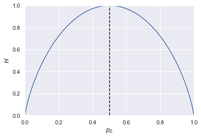
Here we can see that the entropy is maximal for the unbiased coin. This is true in general: the entropy peaks for the uniform distribution. In a sense, this is the most unpredictable distribution: if we get heads with probability 0.2, betting tails is a great idea. On the other hand, if the coin is unbiased, then a deterministic strategy is of little help in winning. Entropy quantifies this notion of surprise and unpredictability.
33. Quantum states
34. Qubits revisited
In the previous we introduced classical probability theories and the stochastic vector, which describes a probability distribution. So, based on that, we can easily introduce quantum states. So a quantum state is just like stochastic vector. You can write it as a column vector.
But the big difference is that you are not restricted to real numbers and nonnegative real numbers, because the entries in this vector are complex values. And the normalization of this vector doesn’t happen in the one norm, it happens in the two norm.
So it’s still normalizing to \(1\), but now the square sum of the absolute values of the entries is what adds up to 1, as opposed to just the absolute values adding up to \(1\).
This is the simplest possible quantum state. It has two possible outcomes. This is often referred to as a qubit.
Finish
A classical coin is a two-level system: it is either heads or tails. At a first look a quantum state is a probability distribution, and the simplest case is a two-level state, which we call a qubit. Just like the way we can write the probability distribution as a column vector, we can write a quantum state as a column vector. For notational convenience that will become apparent later, we write the label of a quantum state in what is called a ket in the Dirac notation. So for instance, for some qubit, we can write
In other words, a ket is just a column vector, exactly like the stochastic vector in the classical case. Instead of putting an arrow over the name of the variable to express that it is a vector, we use the ket to say that it is a column vector that represents a quantum state. There’s more to this notation, as we will see.
The key difference to classical probability distributions and stochastic vectors is the normalization constraint. The square sum of their absolute values adds up to 1:
where $\(a_0, a_1\in \mathbb{C}\)$
In other words, we are normalizing in the \(l_2\) norm instead of the \(l_1\) norm. Furthermore, we are no longer restricted to the positive orthant: the components of the quantum state vector, which we call probability amplitudes, are complex valued.
35. Superposition revisited
And a superposition is just the expansion of this vector in a basis. For instance, if it expanded in the canonical basis, like this, then we can introduce a notation for the \(1 0\) vector and the \(0 1\) vector.
Outcome \(0\) with probability $\(\mid a_{0}\mid^{2}\)$
state afterwards: $\(\mid0\rangle\)$
Now the
is called the 0 ket $\(\mid0\rangle\)$
And the $\(\left[\begin{array}{c}0\\1\end{array}\right]\)$
the second basis vector, is called the 1 ket
And this notation, the vertical bar, and this little angle, often the name of the vector– is ket. This gives us the same idea as in a stochastic vector, that we have to put an arrow on top of the vector, that will help us in the syntax of writing calculations on the quantum states. Here
is the superposition of the \(0\) and the \(1 ket\) , with different coefficients \(a_{0}\) and \(a_{1}\). So these coefficients are called probability amplitudes. They no longer represent probabilities directly, as in the case of a stochastic vector, but it’s the absolute value squared of these values what gives you a probability. So, for instance, you get the outcome 0, with probability a0 squared and, similarly, outcome 1, with probability of the absolute value of a1 squared. And, once you get an outcome 0,
you know that the state is in the 0 state. And similarly, if you get the outcome 1, afterwards the state is going to be in the state 1. This is called the “collapse of the wave function.” A quantum state is also called a wave function. And basically, once you pull out a sample of this distribution and you get an outcome, you make that observation, then you get the deterministic state afterwards, after the random outcome. So you can also think about it in a more geometric way. So now you have a two-dimensional complex space which would take a four dimensions to visualize. But we have this restriction on the degree of freedom. So we can have some three-dimensional object representing these qubit states.
Let us introduce two special qubits, corresponding to the canonical basis vectors in two dimensions: $\(\mid 0\rangle\)\( and \)\(\mid 1\rangle\)$
This basis is also called the computational basis in quantum computing.
We can expand an arbitrary qubit state in this basis:
This expansion in a basis is called a superposition. If we sample the qubit state, we obtain the outcome 0 with probability \(|a_0|^2\), and 1 with probability \(|a_1|^2\). This is known as the Born rule; you will learn more about measurements and this rule in a subsequent notebook.
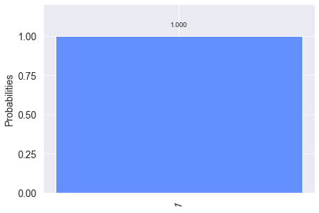
For now, let’s take a look at how we can simulate classical coin tossing on a quantum computer. Let’s start with a completely biased case where we get heads with probability 1. This means that our qubit \(|\psi\rangle=|0\rangle\). We create a circuit of a single qubit and a single classical register where the results of the sampling (measurements) go.
from qiskit import QuantumCircuit, ClassicalRegister, QuantumRegister
from qiskit import execute
from qiskit import BasicAer
from qiskit.tools.visualization import plot_histogram, plot_bloch_multivector

import numpy as np
π = np.pi

backend = BasicAer.get_backend('qasm_simulator')

q = QuantumRegister(1)
c = ClassicalRegister(1)
circuit = QuantumCircuit(q, c)
Any qubit is initialized in \(|0\rangle\), so if we measure it right away, we should get our maximally biased coin.
circuit.measure(q, c)
<qiskit.circuit.instructionset.InstructionSet at 0x10f511390>
Let us execute it a hundred times and study the result
job = execute(circuit, backend, shots=100)
result = job.result()
result.get_counts(circuit)
{'0': 100}
As expected, all of our outcomes are 0.
36. Bloch Sphere revisited
So this is where the Bloch sphere helps us. So Bloch sphere is this three-dimensional sphere, but with a slightly different geometry than a normal sphere. So here the north pole is identified with the 0 ket, and the south pole is identified with the 1 ket.
It’s a little bit unusual, because these two basis vectors are actually orthogonal. And it gives an illusion as if they’re relying on the same line. So just keep in mind that orthogonality is a little bit different in this sphere. And now every single point on the surface of the sphere is a qubit state
So, basically, you have a much larger representative power. If you compare it, for instance, with classical probability distributions, where every single probability distribution lies on this straight line, as opposed to this large, two-dimensional surface of the Bloch sphere. Now, there are a couple of things that we can do with quantum states which we cannot do, for instance, in classical digital computers.
To understand the possible quantum states, we use the Bloch sphere visualization. Since the probability amplitudes are complex and there are two of them for a single qubit, this would require a four-dimensional space. Now since the vectors are normalized, this removes a degree of freedom, allowing a three-dimensional representation with an appropriate embedding. This embedding is the Bloch sphere. It is slightly different than an ordinary sphere in three dimensions: we identify the north pole with the state $\(\mid 0\rangle\)\( and the south pole with \)|1\rangle$. In other words, two orthogonal vectors appear as if they were on the same axis – the axis Z. The computational basis is just one basis: the axes X and Y represent two other bases. Any point on the surface of this sphere is a valid quantum state. This is also true the other way around: every pure quantum state is a point on the Bloch sphere. Here it ‘pure’ is an important technical term and it essentially means that the state is described by a ket (column vector). Later in the course we will see other states called mix states that are not described by a ket (you will see later that these are inside the Bloch sphere).
To make it less abstract, let’s plot our $\(\mid 0\rangle\)$ on the Bloch sphere:
backend_statevector = BasicAer.get_backend('statevector_simulator')
circuit = QuantumCircuit(q, c)
#circuit.iden(q[0])
#QuantumCircuit.iden(q[0])
circuit.id(q[0])
job = execute(circuit, backend_statevector)
plot_bloch_multivector(job.result().get_statevector(circuit))
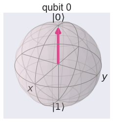
Compare this sphere with the straight line in the positive orthant that describes all classical probability distributions of coin tosses. You can already see that there is a much richer structure in the quantum probability space.
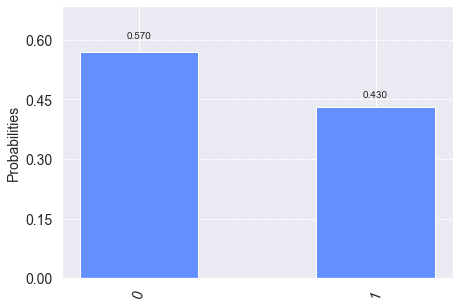
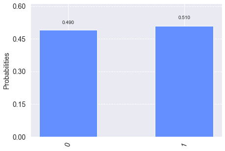
Let us pick another point on the Bloch sphere, that is, another distribution. Let’s transform the state $\(\mid 0\rangle\)\( to \)\(\frac{1}{\sqrt{2}}(|0\rangle + |1\rangle)\)\( This corresponds to the unbiased coin, since we will get 0 with probability \)\(\mid\frac{1}{\sqrt{2}}|^2=1/2\)\( and the other way around. There are many ways to do this transformation. We pick a rotation around the Y axis by \)\pi/2\(, which corresponds to the matrix \)\(\frac{1}{\sqrt{2}}\begin{bmatrix} 1 & -1\\1 & 1\end{bmatrix}\)$
circuit = QuantumCircuit(q, c)
circuit.ry(π/2, q[0])
circuit.measure(q, c)
job = execute(circuit, backend, shots=100)
plot_histogram(job.result().get_counts(circuit))
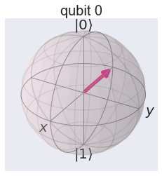
To get an intuition why it is called a rotation around the Y axis, let’s plot it on the Bloch sphere:
circuit = QuantumCircuit(q, c)
circuit.ry(π/2, q[0])
job = execute(circuit, backend_statevector)
plot_bloch_multivector(job.result().get_statevector(circuit))
It does exactly what it says: it rotates from the north pole of the Bloch sphere.
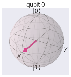
Why is interesting to have complex probability amplitudes instead of non-negative real numbers? To get some insight, take a look what happens if we apply the same rotation to \(|1\rangle\). To achieve this, first we flip \(|0\rangle\) to \(|1\rangle\) by applying a NOT gate (denoted by X in quantum computing) and then the rotation.
circuit = QuantumCircuit(q, c)
circuit.x(q[0])
circuit.ry(π/2, q[0])
job = execute(circuit, backend_statevector)
plot_bloch_multivector(job.result().get_statevector(circuit))
We can verify that the result is $\(\frac{1}{\sqrt{2}}(-|0\rangle + |1\rangle)\)$ That is, the exact same state as before, except that the first term got a minus sign: it is a negative probability amplitude. Note that the difference cannot be observed from the statistics:
circuit.measure(q, c)
job = execute(circuit, backend, shots=100)
plot_histogram(job.result().get_counts(circuit))
37. Interference
Interference is a strange phenomenon where the different basis vectors and the coefficients interact in your calculations.
So imagine that you act on your 0 ket with this particular matrix. Remember that, in your transform stochastic vectors, with matrices, with stochastic matrices, to ensure that the result is also a stochastic vector, a probability distribution, quantum states are also acted on by these operators, and they fulfill certain conditions that we will learn later. Now, just accept that this is a valid operation, and it transform the 0 ket into the equal superposition of the 0 and the 1 ket. And, if you are acting on the 1 ket, the only difference would be that it would introduce a negative sign to the 0 ket.
Interestingly is, if we now take this outcome $\(\frac{1}{\sqrt{2}}(\mid0\rangle+\mid1\rangle)\)$ and we apply the same operation on it– that’s what we are doing here– so I take this outcome, and I apply the same operation on it– then something interesting is happening. So this is a linear operator, so I can pull out the 1 over square root 2 the front, so it simplifies to 1/2. And I can also take the matrix operation basis vector by basis vector in the superposition.
So I act on the first one. From that, I get the superposition of 0 and 1 \(\mid0\rangle+\mid1\rangle\), just like here, the same thing. And then I have the 1 ket, so I’m going to get this outcome, which we calculated here. And now, if you look at this, these two cancel out
Which means that we get a deterministic outcome by applying the operator again. So this is an example of interference. So t he probability amplitudes of the 0 ket destructive interfere, they vanish from the superposition, and you get the deterministic 1 outcome.
37.1. Quiz Quantum States
Is $\(\frac{1}{3}\mid0\rangle+\sqrt{\frac{2}{3}}\mid1\rangle\)$ a valid quantum state?
False
In a quantum state, the probability amplitudes are not restricted to the positive orthant. This is what enables interference.
True
The points on the surface of the Bloch sphere…
are qubit states
It still looks like an approximately unbiased coin. Yet, that negative sign – or any complex value – is what models interference, a critically important phenomenon where probability amplitudes can interact in a constructive or a destructive way. To see this, if we apply the rotation twice in a row on $\(|0\rangle\)\( we get another deterministic output, \)\(1\rangle\)$ although in between the two, it was some superposition.
circuit = QuantumCircuit(q, c)
circuit.ry(π/2, q[0])
circuit.ry(π/2, q[0])
circuit.measure(q, c)
job = execute(circuit, backend, shots=100)
plot_histogram(job.result().get_counts(circuit))
Many quantum algorithms exploit interference, for instance, the seminal Deutsch-Josza algorithm, which is among the simplest to understand its significance.
38. More qubits and entanglement
39. Multiple Qubits revisited
Starting with the simplest possible quantum system, a qubit state and try to construct larger probability distributions, or larger states, which are composed of several qubits. Before we go there, we have to introduce a new mathematical operation, a tensor product. Imagine that you have two quantum states, two kets. One has a probability amplitudes a0 a1, and the second one has b0 and b1.
Now, then, we can define this tensor product as this object.
First we have $\(a_{0} \otimes b_{0}\)\( as the first component, and you have \)\(a_{0} \otimes b_{1}\)\( \)\(a_{1} \otimes b_{0}\)\( which is a four-dimensional complex vector. These are independently two-dimensional complex vectors, and here we create a four-dimensional one. And now we can also look at this probability distribution-- has four possible outcomes. We can create a basis, in this space by taking our \)0\( ket and take the tensor product of the other \)0$ kets.
Convention right most qubit is qubit \(0\)
The shorthand notation for this is just dropping the tensor product sign. Even shorter notation is by dropping the two kets, here, and just contracting them into one. And if we calculate the product, then we end up with the first canonical basis vector of the four-dimensional space. The same thing with 0 and 1, 1 0, and 1 1. Noticing that these are the four possibilities, the four canonical basis vectors, in the four-dimensional complex space. There’s a very important convention that most quantum-computing libraries out there use, which is that it’s the rightmost qubit which is the qubit 0. This would be qubit 0. And then to the left of it would be qubit 1, and so on, and so forth.
This is the same order of representing binary values as you would have in most digital computers, and that’s why this convention is maintained in these quantum-computing frameworks. These are called “product states,” but there are also states which cannot be written in this form, even though they live in the same space. One example is the \(\phi+\) state.
It’s written as an equal superposition of two basis vectors, 0 0 and 1 1, so it’s definitely in the same space as our product vector.
But it cannot be written as a product vector. And, to see that, let’s take a look at the general structure of this product vector.
We copied the definition of the product vector here and wrote it down in the canonical basis. It would have a0 times b0 times the 0 0 ket, and so on. It has four components. And let us assume that there is some combination of these ai and bj values such that we can write this phi plus state as a product state.
So this means that, either here we have 0 0 ket with a coefficient 1 over square root 2– so this equation must be fulfilled.
Similarly, we have the \(1 1\) ket with the same coefficient. This condition must be fulfilled. And we also see that there is no 0 1 and 1 0, so the corresponding coefficient must be 0. But now, it means that either a0 or b1 must be 0. a0 cannot be 0, because it multiplies to some known nonzero value, but the same is true for b1. Therefore the state, although it lives in the same space, cannot be written as a product state. Such states are called “entangled states,” and they play a very important role in quantum computing, together with interference. So these are the main quantum-mechanical properties that we exploit in quantum calculations, as you will see in subsequent lectures.
39.1. Quiz
The \(\mid00\rangle\) state is the same as… $\(\mid0\rangle\otimes\mid0\rangle\)$
– the first basis vector in the canonical basis in four dimensions.
Since the basis of $\(\mathbb{C}^{2}\otimes\mathbb{C}^{2}\)$ is created as product states, all states in this space must be product states.
False
We have already seen that quantum states are probability distributions normed to \(1\) in the \(l_{2}\) norm and we got a first peek at interference. If we introduce more qubits, we see another crucial quantum effect emerging. To do that, we first have to define how we write down the column vector for describing two qubits. Using a tensor product, which, in the case of qubits, is equivalent to the Kronecker product. Given two qubits, $\(\mid\psi\rangle=\begin{bmatrix}a_0\\a_1\end{bmatrix}\)\( and \)\(\mid\psi'\rangle=\begin{bmatrix}b_0\\b_1\end{bmatrix}\)\( their product is \)\(\mid\psi\rangle\otimes\mid\psi'\rangle = \begin{bmatrix}a_0b_0\\ a_0b_1\\ a_1b_0\\ a_1b_1\end{bmatrix}\)\( Imagine that you have two registers \)q_{0}\( and \)q_{1}\( each can hold a qubit, and both qubits are in the state \)\(\mid 0\rangle\)$ Then this composite state would be described by according to this product rule as follows:
q0 = np.array([[1], [0]])
q1 = np.array([[1], [0]])
np.kron(q0, q1)
array([[1],
       [0],
       [0],
       [0]])
This is the \(|0\rangle\otimes|0\rangle\) state, which we often abbreviate as \(|00\rangle\). The states \(|01\rangle\), \(|10\rangle\), and \(|11\rangle\) are defined analogously, and the four of them give the canonical basis of the four dimensional complex space, \(\mathbb{C}^2\otimes\mathbb{C}^2\).
Now comes the interesting and counter-intuitive part. In machine learning, we also work with high-dimensional spaces, but we never construct it as a tensor product: it is typically \(\mathbb{R}^d\) for some dimension \(d\). The interesting part of writing the high-dimensional space as a tensor product is that not all vectors in can be written as a product of vectors in the component space.
Take the following state: \(|\phi^+\rangle = \frac{1}{\sqrt{2}}(|00\rangle+|11\rangle)\). This vector is clearly in \(\mathbb{C}^2\otimes\mathbb{C}^2\), since it is a linear combination of two of the basis vector in this space. Yet, it cannot be written as \(|\psi\rangle\otimes|\psi'\rangle\) for some \(|\psi\rangle\), \(|\psi'\rangle\in\mathbb{C}^2\).
To see this, assume that it can be written in this form. Then
\(|01\rangle\) and \(|10\rangle\) do not appear on the left-hand side, so their coefficients must be zero: \(a_1b_0=0\) and \(a_0b_1=0\). This leads to a contradiction, since \(a_1\) cannot be zero (\(a_1b_1=1\)), so \(b_0\) must be zero, but \(a_0b_0=1\). Therefore \(|\phi^+\rangle\) cannot be written as a product.
States that cannot be written as a product are called entangled states. This is the mathematical form of describing a phenomenon of strong correlations between random variables that exceed what is possible classically. Entanglement plays a central role in countless quantum algorithms. A simple example is quantum teleportation. We will also see its applications in quantum machine learning protocols.
We will have a closer look at entanglement in a subsequent notebook on measurements, but as a teaser, let us look at the measurement statistics of the \(|\phi^+\rangle\) state. The explanation of the circuit preparing it will also come in a subsequent notebook.
q = QuantumRegister(2)
c = ClassicalRegister(2)
circuit = QuantumCircuit(q, c)
circuit.h(q[0])
circuit.cx(q[0], q[1])
circuit.measure(q, c)
job = execute(circuit, backend, shots=100)
plot_histogram(job.result().get_counts(circuit))
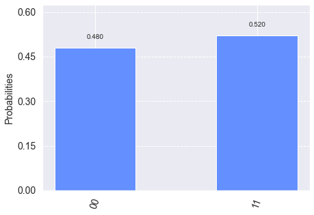
Notice that 01 or 10 never appear in the measurement statistics.
40. Further reading
Chapter 9 in Quantum Computing since Democritus by Scott Aaronson describes a similar approach to understanding quantum states – in fact, the interference example was lifted from there.