41. Measurements revisited
In the previous we introduced quantum states as a generalization of classical probabilities. But we left it open how to exactly extract a certain event with a certain probability. To formalize this, we have to introduce measurements. Prior to introducing measurements, we neet to introduce a bit more of the notation. Remembering that we introduced a quantum state as a column vector, which we write as a ket.
42. Bra-Ket Notation
So we have a vertical bar, and an angle sign, an in-between we write the name of the vector or the variable. And in the simplest case, this is a two-level system, it’s a qubit, so it can take– it’s a vector of two elements, and both elements are complex. Now, a complex number, in general, is written in this form.
\(a_{0} =x_{0}+iy_{0}\)
So for instance, \(a_{0}\) is equal to \(x_{0}\), which is a real number, plus the imaginary number times \(y_0\). Now, there is something that we can do with complex numbers that we cannot do with real numbers– we can take their conjugate. Which means that we flip the sign of the imaginary component. So with this conjugate we can introduce the complement of a ket.
\(\bar{a_{0}}=x_{0}-iy_{0}\) Which is its conjugate transpose. So it’s called a bra. And it’s written as the mirror of the ket. So we start in an angle side from the other side, and then we write a name of the bra, and then a vertical sign. So this is equal to the complex conjugate transpose of the ket. This sign is called a dagger.
\(\text{Bra:}\langle\psi\mid=\mid\psi\rangle^{\dagger}=\left[\bar{a_{0}}\bar{a_{1}}\right]\)
And since this is a transpose, it’s going to be a row vector. And each of the complex components is going to take its complex conjugate. So that’s it.
43. Dot product
So you can think of it as when we talk about stochastic vectors, we can also transpose them. But since we talk about real numbers, in the case of stochastic vectors, this complex component doesn’t make any sense. Whereas here, we have to take care that we deal with complex numbers and there’s something to get out of this. So for instance, with this notation it’s very easy to write dot productions. So for instance, if we take the bra of some arbitrary state side, and we follow it up by a ket, that’s going to be the product of a row vector with a column vector. In other words, it’s going to be a dot product.
It expands as the absolute value of \(a_{0}\) squared plus the absolute value of \(a_{1}\) squared. And we know that since the vector is normalized this is just 1. So there’s just one particular way of writing the two norm– by the square of the 2 norm of the quantum state.
And for instance, if you look at the 0 ket and it’s dot product with the 1 ket, then what we’re going to do is we take this row vector multiply it by this column vector, and that’s going to be 0. And it’s not surprising, because the dot product of orthogonal vectors is always zero. So what if we take the other order. So we take the ket and the bra. So you see this is a bra and this is a ket, which gives you a scalar.
44. Ket-Bra
If we take a ket and a bra, which we also write in this form– it’s just easier to write– there’s not going to be a scalar, this is going to be a matrix.
In this case, we are multiplying this column vector with this vector, which is going to give you this matrix. So the order makes a big difference. If you take a ket and a bra, that gives you a matrix. But if you take a bra and a ket, that gives you a scalar value. And as a matter of fact, if you look at this carefully, this is nothing else but the projection to this particular basis vector. So armed with this knowledge, we can, start talking about measurements. So the intuition is that the measurement is very, very similar to a random variable in classical probability theory. So in classical probability theory random variables take values. And here measurements, take measurement outcomes. And you always get a random outcome, just the same way random variables is intrinsically random.
A measurement is a central concept in quantum mechanics. An easy way to think about it as a sample from a probability distribution: it is a random variable with a number of outcomes, each outcome is produced with a certain probability.
Measurement connect the quantum world to our classical one: we cannot directly observe the quantum state in nature, we can only gather statistics about it with measurements. It sounds like a harsh boundary between a quantum and a classical system that can only be bridged by measurement. The reality is more subtle: unless a quantum system is perfectly isolated, it interacts with its surrounding environment. This leads to introduction of mixed states, which in one limit recover classical probabilities.
45. More on the bra-ket notation
Before we deep dive into what measurements are, we need to introduce one more notation to complement the ket: it called a bra and it is denoted by $\(\langle\psi|\)\( for some quantum state \)\(\mid\psi\rangle\)\( Together they form the bra-ket or Dirac notation. A bra is the conjugate transpose of a ket, and the other way around. This also means that a bra is a row vector. For instance, this is the bra for \)\(\mid0\rangle\)$
import numpy as np
zero_ket = np.array([[1], [0]])
print("|0> ket:\n", zero_ket)
print("<0| bra:\n", zero_ket.T.conj())
|0> ket:
 [[1]
 [0]]
<0| bra:
 [[1 0]]
This makes it very easy to write dot products: if we write a bra followed by a ket, that is exactly what the dot product is. This is so common that we often drop one of the vertical bars, and just write \(\langle 0|0\rangle\), for instance. Since quantum states are normalized, the inner product of any quantum state with itself is always one:
zero_ket.T.conj() @ zero_ket
array([[1]])
Similarly, orthogonal vectors always give 0. E.g. \(\langle 0|1\rangle\):
one_ket = np.array([[0], [1]])
zero_ket.T.conj() @ one_ket
array([[0]])
What about a ket and a bra? That is going to be a matrix: essentially the outer product of the two vectors. Here’s \(|0\rangle\langle 0|\):
zero_ket @ zero_ket.T.conj()
array([[1, 0],
       [0, 0]])
This should look familiar: it is a projection to the first element of the canonical basis. It is true in general that \(|\psi\rangle\langle\psi|\) is going to be a projector to \(|\psi\rangle\). It is very intuitive: take some other quantum state \(|\phi\rangle\) and apply the matrix \(|\psi\rangle\langle\psi|\) on it: \(|\psi\rangle\langle\psi|\phi\rangle\). Now the right-most two terms are a bra and a ket, so it is a dot product: the overlap between \(|\phi\rangle\) and \(|\psi\rangle\). Since this is a scalar, it just scales the left-most term, which is the ket \(|\psi\rangle\), so in effect, we projected \(|\phi \rangle\) on this vector.
46. More on Measurements
A measurement in quantum mechanics is an operator-valued random variable. The theory of measurements is rich and countless questions about them are still waiting to be answered. Most quantum computers that we have today, however, only implement one very specific measurement, which makes our discussion a lot simpler. This measurement is in the canonical basis. In other words, the measurement contains two projections, $\(\mid0\rangle\langle 0\mid\)\( and \)\(\mid1\rangle\langle 1\mid\)$ and this measurement can be applied to any of the qubits of the quantum computer.
We already saw how applying a projection on a vector works. If we want to make a scalar value of that, we need to add a bra to the left. For instance, for some state $\(\mid\psi\rangle\)\( we get a scalar for \)\(\langle\psi|0\rangle\langle 0|\psi\rangle\)\( This is called the expectation value of the operator \)\(\mid0\rangle\langle 0\mid\)\( To put this in context, let us apply the projection \)\(\mid0\rangle\langle 0\mid\)\( on the superposition \)\(\frac{1}{\sqrt{2}}(|0\rangle + \mid1\rangle)\)\( which is the column vector \)\(\frac{1}{\sqrt{2}}\begin{bmatrix} 1\\ 0\end{bmatrix}\)$
ψ = np.array([[1], [0]])/np.sqrt(2)
Π_0 = zero_ket @ zero_ket.T.conj()
ψ.T.conj() @ Π_0 @ ψ
array([[0.5]])
#!pip install qiskit==0.16.1
!pip install qiskit
Requirement already satisfied: qiskit in /Users/moh/micromamba/envs/mom1env/lib/python3.8/site-packages (0.43.1)
Requirement already satisfied: qiskit-terra==0.24.1 in /Users/moh/micromamba/envs/mom1env/lib/python3.8/site-packages (from qiskit) (0.24.1)
Requirement already satisfied: qiskit-aer==0.12.0 in /Users/moh/micromamba/envs/mom1env/lib/python3.8/site-packages (from qiskit) (0.12.0)
Requirement already satisfied: qiskit-ibmq-provider==0.20.2 in /Users/moh/micromamba/envs/mom1env/lib/python3.8/site-packages (from qiskit) (0.20.2)
Requirement already satisfied: numpy>=1.16.3 in /Users/moh/micromamba/envs/mom1env/lib/python3.8/site-packages (from qiskit-aer==0.12.0->qiskit) (1.23.5)
Requirement already satisfied: scipy>=1.0 in /Users/moh/micromamba/envs/mom1env/lib/python3.8/site-packages (from qiskit-aer==0.12.0->qiskit) (1.10.1)
Requirement already satisfied: requests>=2.19 in /Users/moh/micromamba/envs/mom1env/lib/python3.8/site-packages (from qiskit-ibmq-provider==0.20.2->qiskit) (2.31.0)
Requirement already satisfied: requests-ntlm<=1.1.0 in /Users/moh/micromamba/envs/mom1env/lib/python3.8/site-packages (from qiskit-ibmq-provider==0.20.2->qiskit) (1.1.0)
Requirement already satisfied: urllib3>=1.21.1 in /Users/moh/micromamba/envs/mom1env/lib/python3.8/site-packages (from qiskit-ibmq-provider==0.20.2->qiskit) (2.0.3)
Requirement already satisfied: python-dateutil>=2.8.0 in /Users/moh/micromamba/envs/mom1env/lib/python3.8/site-packages (from qiskit-ibmq-provider==0.20.2->qiskit) (2.8.2)
Requirement already satisfied: websocket-client>=1.5.1 in /Users/moh/micromamba/envs/mom1env/lib/python3.8/site-packages (from qiskit-ibmq-provider==0.20.2->qiskit) (1.6.0)
Requirement already satisfied: websockets>=10.0 in /Users/moh/micromamba/envs/mom1env/lib/python3.8/site-packages (from qiskit-ibmq-provider==0.20.2->qiskit) (11.0.3)
Requirement already satisfied: rustworkx>=0.12.0 in /Users/moh/micromamba/envs/mom1env/lib/python3.8/site-packages (from qiskit-terra==0.24.1->qiskit) (0.13.0)
Requirement already satisfied: ply>=3.10 in /Users/moh/micromamba/envs/mom1env/lib/python3.8/site-packages (from qiskit-terra==0.24.1->qiskit) (3.11)
Requirement already satisfied: psutil>=5 in /Users/moh/micromamba/envs/mom1env/lib/python3.8/site-packages (from qiskit-terra==0.24.1->qiskit) (5.9.5)
Requirement already satisfied: sympy>=1.3 in /Users/moh/micromamba/envs/mom1env/lib/python3.8/site-packages (from qiskit-terra==0.24.1->qiskit) (1.12)
Requirement already satisfied: dill>=0.3 in /Users/moh/micromamba/envs/mom1env/lib/python3.8/site-packages (from qiskit-terra==0.24.1->qiskit) (0.3.6)
Requirement already satisfied: stevedore>=3.0.0 in /Users/moh/micromamba/envs/mom1env/lib/python3.8/site-packages (from qiskit-terra==0.24.1->qiskit) (5.1.0)
Requirement already satisfied: symengine<0.10,>=0.9 in /Users/moh/micromamba/envs/mom1env/lib/python3.8/site-packages (from qiskit-terra==0.24.1->qiskit) (0.9.2)
Requirement already satisfied: six>=1.5 in /Users/moh/micromamba/envs/mom1env/lib/python3.8/site-packages (from python-dateutil>=2.8.0->qiskit-ibmq-provider==0.20.2->qiskit) (1.16.0)
Requirement already satisfied: charset-normalizer<4,>=2 in /Users/moh/micromamba/envs/mom1env/lib/python3.8/site-packages (from requests>=2.19->qiskit-ibmq-provider==0.20.2->qiskit) (3.1.0)
Requirement already satisfied: idna<4,>=2.5 in /Users/moh/micromamba/envs/mom1env/lib/python3.8/site-packages (from requests>=2.19->qiskit-ibmq-provider==0.20.2->qiskit) (3.4)
Requirement already satisfied: certifi>=2017.4.17 in /Users/moh/micromamba/envs/mom1env/lib/python3.8/site-packages (from requests>=2.19->qiskit-ibmq-provider==0.20.2->qiskit) (2023.5.7)
Requirement already satisfied: ntlm-auth>=1.0.2 in /Users/moh/micromamba/envs/mom1env/lib/python3.8/site-packages (from requests-ntlm<=1.1.0->qiskit-ibmq-provider==0.20.2->qiskit) (1.5.0)
Requirement already satisfied: cryptography>=1.3 in /Users/moh/micromamba/envs/mom1env/lib/python3.8/site-packages (from requests-ntlm<=1.1.0->qiskit-ibmq-provider==0.20.2->qiskit) (41.0.1)
Requirement already satisfied: pbr!=2.1.0,>=2.0.0 in /Users/moh/micromamba/envs/mom1env/lib/python3.8/site-packages (from stevedore>=3.0.0->qiskit-terra==0.24.1->qiskit) (5.11.1)
Requirement already satisfied: mpmath>=0.19 in /Users/moh/micromamba/envs/mom1env/lib/python3.8/site-packages (from sympy>=1.3->qiskit-terra==0.24.1->qiskit) (1.3.0)
Requirement already satisfied: cffi>=1.12 in /Users/moh/micromamba/envs/mom1env/lib/python3.8/site-packages (from cryptography>=1.3->requests-ntlm<=1.1.0->qiskit-ibmq-provider==0.20.2->qiskit) (1.15.1)
Requirement already satisfied: pycparser in /Users/moh/micromamba/envs/mom1env/lib/python3.8/site-packages (from cffi>=1.12->cryptography>=1.3->requests-ntlm<=1.1.0->qiskit-ibmq-provider==0.20.2->qiskit) (2.21)
That is exactly one half, the square of the absolute value of the probability amplitude corresponding to \(|0\rangle\) in the superposition! This is the mathematical formalism of what we had said earlier: given a state \(|\psi\rangle = a_0|0\rangle + a_1|1\rangle\), we get an output \(i\) with probability \(|a_i|^2\). This is known as the Born rule. Now we have a recipe to extract probabilities with projections. This is exactly what is implemented in the quantum simulator. The measurement in the simulator is what we described here. Let’s create an equal superposition with the Hadamard gate (see a later notebook for quantum circuits), apply the measurement, and observe the statistics:
from qiskit import QuantumCircuit, ClassicalRegister, QuantumRegister
from qiskit import execute
from qiskit import BasicAer as Aer
from qiskit.tools.visualization import plot_histogram

backend = Aer.get_backend('qasm_simulator')
q = QuantumRegister(1)
c = ClassicalRegister(1)
circuit = QuantumCircuit(q, c)
circuit.h(q[0])
circuit.measure(q, c)
job = execute(circuit, backend, shots=100)
plot_histogram(job.result().get_counts(circuit))
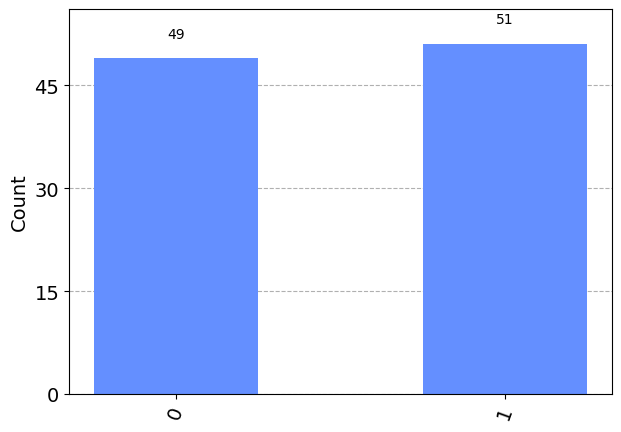
You see that the outcome is random, with roughly half of the outcomes being 0.
47. Collapse of the Wave Function
To make it more formal, if we remember the mentioned the Born Rule, which tells you that you get some outcomes 0 of the qubit state with probability the absolute value of $\(\mid a_{0}\mid^{2}\)$
And the state afterwards becomes the 0 ket \mid0\rangle collapse of the wave function . So the superposition is destroyed and you only get one part of the superposition. This is random which part you get with a certain probability, but this is what we call the collapse of the wave function. And the way we write it down is actually with this formalism. So the measurement outcome is actually a projection.
So for instance, if you want to model that we get the outcome 0, then we take the corresponding projection and we apply it on the quantum state.
Now, if we look at this carefully, this is a ket and a bra. It’s just the bra and the ket, which means that this is going to be a scalar in fact this is just the projection to this particular basis vector. So this is going to be the 0 ket times A0.
And if you take the absolute value, we take the length of this vector that’s going to be exactly this vector. So if we take the length of A0 time the 0 ket squared, that’s going to give you exactly what the Born Rule tells you. And now if you look at this expression $\(\mid\mid a_{0}\mid0\rangle\mid\mid_{2}^{2}\)\( and you look at this expression \)\(\mid0\times0\mid\)$ you know that you can write the square of the two norm in this form. So we can actually write this as say, this.
Or in other words, we can also look at it as an expectation of value of this outcome. And the state afterwards is basically this state just renormalized. Which means that if we look at what we get, this is going to be this projection in the nominator, and in the denominator we have to renormalize this state, which is going to be the square root of exactly this expression.
48. The Born Rule
This is the mathematical way of describing how you pull out samples from a quantum state, and otherwise how we apply measurements to this particular probability distribution.
https://en.wikipedia.org/wiki/Born_rule:
The Born rule (also called the Born law, Born’s rule, or Born’s law), formulated by German physicist Max Born in 1926, is a physical law[citation needed] of quantum mechanics giving the probability that a measurement on a quantum system will yield a given result.[1] In its simplest form it states that the probability density of finding the particle at a given point is proportional to the square of the magnitude of the particle’s wavefunction at that point.
48.1. Measurements Quiz
Checkboxes:
A bra \(\langle\psi\mid\) is
a row vector
– The conjugate transpose of the ket $\(\mid\psi\rangle\)$
The Born rule tells us
what is the probability of getting an output and
what the state is after the measurement.
By applying the projection $\(\mid0\rangle\langle0\mid\)\( on the state \)\(\frac{\left(\mid0\rangle+\mid1\rangle\right)}{\sqrt{2}}\)$ we get
There is something additional happening. The measurement has a random outcome, but once it is performed, the quantum state is in the corresponding basis vector. That is, the superposition is destroyed. This is referred to as the collapse of the wavefunction. It is the subject of many ongoing debates and research results how and why it happens, but what matters to us is that we can easily calculate the quantum state after the measurement. Just projecting it to the basis vector is insufficient, since that would not be normalized, so we have to renormalize it. Mathematically it is expressed by the somewhat convoluted expression $\(\frac{|i\rangle\langle i|\psi\rangle}{\sqrt{\langle\psi|i\rangle\langle i|\psi\rangle}}\)\( if we observe the output \)i\(. For instance, if we observe zero after measuring the superposition \)\(\frac{1}{\sqrt{2}}(|0\rangle + |1\rangle)\)$ the state after the measurement will be
ψ = np.array([[np.sqrt(2)/2], [np.sqrt(2)/2]])
Π_0 = zero_ket @ zero_ket.T.conj()
probability_0 = ψ.T.conj() @ Π_0 @ ψ
Π_0 @ ψ/np.sqrt(probability_0)
array([[1.],
       [0.]])
which is just a very long way of saying we get \(|0\rangle\).
You can easily see this by putting two measurements in a sequence on the same qubit. The second one will always give the same outcome as the first. The first one is random, but the second one will be determined, since there will be no superposition in the computational basis after the first measurement. Let’s simulate this by writing out the results of the two measurements into two different classical registers:
backend = Aer.get_backend('qasm_simulator')
c = ClassicalRegister(2)
circuit = QuantumCircuit(q, c)
circuit.h(q[0])
circuit.measure(q[0], c[0])
circuit.measure(q[0], c[1])
job = execute(circuit, backend, shots=100)
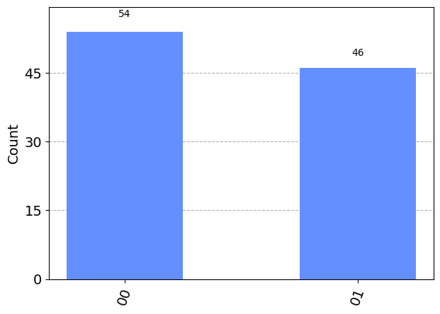
job.result().get_counts(circuit)
{'00': 54, '11': 46}
There is no output like 01 or 10.
49. Measuring multiqubit systems
Most quantum computers implement local measurements, which means that each qubit is measured separately. So if we have a two qubit system where the first qubit is in the equal superposition and the second one is in \(|0\rangle\), that is, we have the state \(\frac{1}{\sqrt{2}}(|00\rangle + |01\rangle)\), we will observe 0 and 0 as outcomes of the measurements on the two qubits, or 0 and 1.
50. Mixed States
Quantum computers we have today are not idealized. To better understand noises and how it affects quantum states, a bit more notation needs to be introduced. This section will address mixed states and which elements in noise affecting quantum computers.
Kets that represent a quantum state are technically speaking also called a pure quantum state. An entirely equivalent notation to pure quantum states is called a Bezoutian matrix, which is a ket and the bra of this quantum state.
We can rewrite every single operation that we would otherwise do in a ket in this formalism. For instance, to get the probability of the outcome 0 can be written as$\(\text{Tr}\left[\mid0\rangle\langle0\mid\rho\right]\)$
51. Density Matrix
We apply the same projection as we applied in our ket, but this time we apply it on this row density matrix. And instead of the length, the normal of this vector, we take the trace of this matrix. So we apply this matrix on this matrix, the outcome is a matrix, and we calculate a trace of it which is the sum of its diagonal elements. So why do we need these density matrices? Why do we need this alternative formalism? Well, the reason is, because we can also create probabilistic mixtures over pure states.
So now you can have the same ket and bra description of a pure quantum state but. You cannot create a classical probability distribution over them. So this p_{i} is classical ignorance. This is something that we don’t know about the underlying quantum system. And if you use this formalism, now we can introduce noise and start making these noisy, imperfect quantum states. And to illustrate the difference, think about this ket
, which is the equal superposition of zero and 1. If we write out the vector form, this is just 1 or squared root 2 in both elements. And if we write the corresponding row, then if you have 1/2 for every element in the matrix. On the other hand, if you create the uniform distribution over the density matrix corresponding to the 0 ket and the density matrix corresponding to the 1 ket, this density matrix will be different.
It will not have off-diagonal elements.
So these off-diagonal elements are critical for many quantum operations. These are sometimes also called coherences. And as you can see, this density matrix does not have any of these and that the diagonal elements are also equal. So this is not just the mixed state, this is called a maximally mixed it. And a maximally mixed state is the equivalent of a uniform distribution in classical probability theory. This means that we have absolutely no predictive power of what’s going to happen next. So in that sense, the entropy of the state is maximal. So ideally, we want quantum states with a high coherence. But in reality, noise effects and these coherences disappear. So let’s take a detour and let’s take a look at what happens when we measure individual qubits in a multi-qubit system.
So imagine that we have the maximally entangled state over 2 qubits, which is written in this form.
And we measure the \(0\) qubit,
which is, according to our notation or convention, is the rightmost qubit. So if we measure this and we get the outcome 0, we moderate it in this form. So this is the measurement operator– just the projection to the first basis vector. And we are not doing anything on this qubit. And we model it by applying the identity matrix on it.
So in this case, this is just 2 by 2 in this form. This means that we are not doing anything on the qubit. And we apply this on this state. So the state collapses from the superposition, and then you get this outcome. So now, if you measure the state again but now the other qubit, you would get 0 deterministically. So this is an entangled state. It exhibits this very strong form of correlation. So even though it just measure 1/2 half, better to get 0 or 1. If you measure the other one, it will be already determined. So let’s take a look at what happens if we are interested in the marginal probability. So this state is like a probability distribution of two random variables. And if you know that we have a multivariate probability distribution, we can marginalize out one of our random variables. We can do the exact same thing in a quantum system by using something called the partial trace.
So imagine that we write our maximally entangled state as a density matrix. You see that it has strong coherences here, although it’s full of 0s– that doesn’t matter. And the way we define partial trace is, imagine if you have any matrix. Here I have a four by four matrix, and you trace out some subpart of it. That operation is defined here as this. So there are elements that you completely get rid of. This corresponds to the random variable that you marginalize out. And then you sum these corresponding diagonal elements to get the final output. So this is the equivalent of marginalizing of the probability distribution. And if you apply this partial trace, say, in the first qubit on our maximally entangled state, what you actually get is the maximally mixed state. This means that if we marginalize out on one of the qubits in this system, then we end up with a uniform distribution. We have absolutely no predictive power over what is going to happen in that remaining quantum system.
• A pure state is one that is described by some ket \mid\psi\rangle , or equivalently, by a density matrix $\(\rho=\mid\psi\rangle\langle\psi\mid\)$ . This means that..
– there is no classical uncertainty about the underlying state.
• The $\(\frac{\boldsymbol{I}}{2}\left[\begin{array}{cc} 0.5 & 0\\ 0 & 0.5 \end{array}\right]\)$ describes a mixed-state qubit..
– True
• By tracing out a subsystem of a pure state, you…
– might end up with a mixed state.
– you take the marginal probability distribution over one variable.
q = QuantumRegister(2)
c = ClassicalRegister(2)
circuit = QuantumCircuit(q, c)
circuit.h(q[0])
circuit.measure(q, c)
job = execute(circuit, backend, shots=100)
plot_histogram(job.result().get_counts(circuit))
What happens if we make measurements on an entangled state? Let’s look at the statistics again on the \(|\phi^+\rangle\) state:
q = QuantumRegister(2)
c = ClassicalRegister(2)
circuit = QuantumCircuit(q, c)
circuit.h(q[0])
circuit.cx(q[0], q[1])
circuit.measure(q, c)
job = execute(circuit, backend, shots=100)
plot_histogram(job.result().get_counts(circuit))
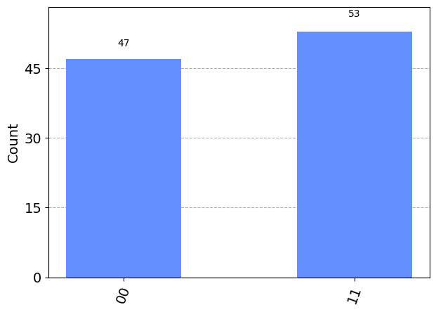
We only observe 00 and 11. Since the state is \(\frac{1}{\sqrt{2}}(|00\rangle+|11\rangle)\), this should not come as a shock. Yet, there is something remarkable going on here. At the end of the last section, we saw the same statistics, but from measurements on the same qubit. Now we have two, spatially separate qubits exhibiting the same behaviour: this is a very strong form of correlations. This means that if we measure just one qubit, and get, say, 0 as the outcome, we know with certainty that if we measured the other qubit, we would also get 0, even though the second measurement is also a random variable.
To appreciate this better, imagine that your are tossing two unbiased coins. If you observe heads on one, there is absolutely nothing that you can say about what the other one might be other than a wild guess that holds with probability 0.5. If you play foul and you biased the coins, you might improve your guessing accuracy. Yet you can never say with certainty what the other coin will be based on the outcome you observed on one coin, except for the trivial case when the other coin deterministically gives the same face always.
Remarkable as it is, there is no activation or instantaneous (faster than the speed of light) signalling happening between the qubits, though. Your measurement was local to the qubit and so is your information. If there is somebody else doing the measurement on the other qubit, you would have to inform the person through classical communication channels that you happen to know what the outcome will be. So while we certainly cannot violate the theory of relativity with entanglement, this strong form of correlation is still central to many quantum algorithms.
ψ = np.array([[1], [1]])/np.sqrt(2)
ρ = ψ @ ψ.T.conj()
Π_0 = zero_ket @ zero_ket.T.conj()
np.trace(Π_0 @ ρ)
0.4999999999999999
We get one half again. The renormalization after a measurement happens in a similar way: \(\frac{|0\rangle\langle 0|\rho|0\rangle\langle 0|}{\mathrm{Tr}[|0\rangle\langle 0|\rho]}\).
probability_0 = np.trace(Π_0 @ ρ)
Π_0 @ ρ @ Π_0/probability_0
array([[1., 0.],
       [0., 0.]])
So why do we need this at all? Every state we have mentioned so far is called a pure state: these are kets or a density matrix created as a ket and a bra. There are other states called mixed states: these are classical probability distributions over pure states. Formally, a mixed state is written as \(\sum_i p_i |\psi_i\rangle\langle\psi_i|\), where \(\sum_i p_i=1\), \(p_i\geq 0\). This reflects our classical ignorance over the underlying quantum states. Compare the density matrix of the equal superposition \(\frac{1}{\sqrt{2}}(|0\rangle+|1\rangle)\) and the mixed state \(0.5(|0\rangle\langle 0|+|1\rangle\langle 1|)\):
zero_ket = np.array([[1], [0]])
one_ket = np.array([[0], [1]])
ψ = (zero_ket + one_ket)/np.sqrt(2)
print("Density matrix of the equal superposition")
print(ψ @ ψ.T.conj())
print("Density matrix of the equally mixed state of |0><0| and |1><1|")
print((zero_ket @ zero_ket.T.conj()+one_ket @ one_ket.T.conj())/2)
Density matrix of the equal superposition
[[0.5 0.5]
 [0.5 0.5]]
Density matrix of the equally mixed state of |0><0| and |1><1|
[[0.5 0. ]
 [0.  0.5]]
The off-diagonal elements are gone in the second case. The off-diagonal elements are also called coherences: their presence indicates that the state is quantum. The smaller these values are, the closer the quantum state is to a classical probability distribution.
The second density matrix above has only diagonal elements and they are equal: this is the equivalent way of writing a uniform distribution. We know that the uniform distribution has maximum entropy, and for this reason, a density matrix with this structure is called a maximally mixed state. In other words, we are perfectly ignorant of which elements of the canonical basis constitute the state.
We would like a quantum state to be perfectly isolated from the environment, but in reality, the quantum computers we have today and for the next couple of years cannot achieve a high degree of isolation. So coherences are slowly lost to the environment – this is a process called decoherence. The speed at which this happens determines the length of the quantum algorithms we can run on the quantum computer: if it happens fast, we have time to apply a handful gates or do any other form calculation, and then we quickly have to pull out (measure) the results.